Introduction
The transformer architecture is the building block for GPT, which contains multiple transformer blocks stacked on top of each other. The transformer processes input sequences through a stack of layers, consisting of a multihead self-attention block and a feed forward neural network. In self-attention, each token in the sequence is broken down into query, key, value vectors, which are used to compute an attention score that determines how much each token attends to every other token. By stacking many of these attention and feed forward layers, transformers build increasingly abstract representations of the input sequence (1).
Large Language Models (LLMs) use these transformer building blocks for natural language processing, but their computational demands pose challenges for inference on models with larger context sizes. Autoregressive transformers like GPT-2 generate text by predicting one token at a time, using attention layers where the current token attends to all previously generated tokens at each step. This causes autoregressive models to do O(n^2) computations to generate a sequence of length n. As context windows for tokens grow in LLMs, this quadratic scaling becomes a critical issue for scaling LLMs for inference tasks.
Pruning is a popular technique to reduce the size of LLMs while maintaining performance. For example, head pruning prunes heads in the multi-headed attention layers of transformers (2). Another approach we consider in this research is reducing the computational cost through token pruning, which removes tokens that contribute little to downstream predictions to reduce the number of attention computations and overall FLOPs done at each layer. Determining which tokens to prune proves to be a more challenging task. A naive implementation looks to remove common function words like "the" and "a" since they appear more frequently and carry less semantic context. However, token importance is not a static property and depends on context, position and layer depth.
This raises a fundamental research question: can we learn to dynamically identify and prune unimportant tokens during inference, reducing computation while preserving generation quality? In this work, we investigate whether integrating two different pruning methods, one based on supervised learning and the other on reinforcement learning, into an autoregressive GPT-2 model can maintain or improve model accuracy while reducing the number of FLOPs
Related Works
We looked at existing works on token pruning with the goal of reducing the tokens passed through each layer during training and inference.
Our initial thought to reduce token usage was pruning "unimportant" tokens in input sequences as they were passed in layer by layer, but determining which tokens were deemed not useful proves to be a much more challenging task. Pruning a static vocabulary of common tokens like "the", "to", and "as" degrades performance since they serve an important role in the English language (3). To avoid this problem, we chose to train a model to learn which tokens are "unimportant".
Another approach uses Learned Token Pruning (LTP), (4) which adaptively removes unimportant tokens from an input sequence as it passes through the transformer layers. LTP works by introducing a new threshold value parameter to each layer. In this case, since we use a 12 layer GPT-2 architecture, there are 12 additional parameters on top of the existing 124M from GPT-2. LTP prunes tokens with attention scores below the threshold value. To define more clearly, we can use the following attention probability equation.
Define the importance score of token x_i in layer l as:
Another possible pruning method involves reinforcement learning using Dynamic Token Reduction (5) by addressing the same quadratic complexity in transformer architectures. This form of learning applies a token reduction module at specified layers. It learns a policy for whether or not to keep each token in a layer. The reward policy equation:
The first term is the log probability of predicting the correct token. The second term subtracts a regularizer multiplied by how many tokens were kept. This equation rewards the model every time it predicts the correct token while keeping a small amount of tokens.
While LTP and Dynamic Token Reduction demonstrate significant efficiency improvements, they were evaluated on a BERT architecture, an encoder-only bidirectional transformer. Autoregressive models like GPT present extra challenges during token pruning because of the causal masking – future tokens can't attend to previous tokens. There hasn't been much prior work that has explored combining supervised learning pruning with RL-based methods.
Methodology and Experiments
Experimental Setup
All experiments use WikiText-2 (raw) language modeling dataset, prepared with GPT-2 BPE tokens for use with NanoGPT. The training set used 2,415,651 tokens while the validation set used 249,750 tokens. We chose this dataset because of its manageable size, which allows for fast training on pruning methods.
Experiments were conducted on a single NVIDIA RTX 5070 Ti. Fine tuning the baseline model took around 5 minutes, while finetuning models with pruning methods took around 10 minutes due to the extra complexity of policy training and threshold learning.
We used the AdamW optimizer, with β1=0.9, β2=0.95, and weight decay of 0.1 to prevent overfitting. For more stable reinforcement learning training, gradient clipping was applied at norm 1.0 to prevent exploding gradients. All models used a cosine learning rate schedule and warmup iterations. We summarize the hyperparameters used for fine tuning in the following table.
| Hyperparameter | Baseline | DTR | LTP | Hybrid |
|---|---|---|---|---|
| Learning Rate | 3e-4 | 1e-4 (Stage 2) | 3e-4 | 3e-4 (LTP), 1e-5 (RL) |
| Batch Size | 8 | 8 | 8 | 8 |
| Sequence Length | 512 | 512 | 512 | 512 |
| Gradient Accumulation | 8 | 8 | 8 | 8 |
| Max Iterations | 300 | 300 | 300 | 300 (LTP), 500 (RL) |
| Warmup Iterations | 100 | 50 | 30 | 30-100 |
| Weight Decay | 0.01 | 0.01 | 0.01 | 0.01 |
| Dropout | 0.0 | 0.0 | 0.0 | 0.0 |
The metrics we report include validation loss, perplexity, average keep ratio, and effective FLOPs (the theoretical computation accounting for pruned tokens). We use the python tool THOP to calculate FLOPs for each layer of our baseline model. During training for our pruning models we collected the fraction of tokens that survive on each layer. We then defined the effective FLOPs for a layer to be:
For the whole model:
We don't actually change the FLOPs calculated by PyTorch in our experiments, but the effective FLOPs calculate how many FLOPs we would have if we did.
Baseline
We use GPT-2 small as our model that we experimented with. It is a 12 layer autoregressive model with around 124 million parameters. Each layer consists of a multi-head self attention block with 12 attention heads and a feed forward network that expands the hidden state dimension of 768 to 3072 before projecting back. We chose to use the small model because it is sufficiently complex, allowing semantics to be captured while retaining the benefits of faster training to run pruning experiments. Our implementation is based on the NanoGPT repository, which implements the GPT-2 architecture and training code.
We decided to fine-tune a pre-trained GPT-2 model on WikiText-2 for our experiments. We fine-tuned the model for 300 training steps and stored this baseline in a checkpoint locally. After fine-tuning we ended with around a 3.1 validation loss. This baseline checkpoint is used for all pruning experiments and as the initialization point for the token reduction models.
Dynamic Token Reduction (DTR) Implementation
The core idea of DTR is to learn a policy network that determines whether to keep or discard each token from the layer. This method of pruning from Ye et. al. was implemented on BERT with backbone freezing and unfreezing. We implemented dynamic token reduction on our baseline GPT-2 model finetuned with WikiText-2. We applied our DTR weights over our frozen baseline for fine-tuning our token reduction policy.
Modifications were made to the GPT architecture. We attach a policy network, a 2-layer MLP that takes the hidden state of each token and outputs a probability for skipping or selecting the token. The policy network can be summarized by the following equation:
During training, we sample a Bernoulli action where selected tokens are kept, and skipped tokens are "pruned". Once a token is pruned at one layer, it remains pruned in subsequent layers.
We use a similar reward equation to the one TR-BERT used. We base this reward off the log probability the token is correct minus the scaled fraction of selected tokens, which effectively separates the reward function into two terms. The first part is the prediction accuracy, which measures a model's performance. The second part is the token reduction penalty term, which acts as a penalty for selecting too many tokens.
where -L_LM is the cross entropy loss, λ=10−4 controls the sparsity penalty, and T is the sequence length.
We defined the policy loss as the negative expectation of the difference of the current reward to the mean reward across the batch multiplied by the summed log probabilities of all sampled/skipped actions.
The total training objective loss combines the language modeling loss with the scaled policy loss.
During training we initially didn't choose a good \alpha, so the policy term dominated and caused the total loss to be unstable and negative. Eventually we found that 0.1 was a good value that encouraged pruning but didn't overwhelm the objective. This caused our reinforcement learning to stabilize and produce meaningful results.
Learned Token Pruning (LTP) Implementation
This method was also implemented on BERT, but we adapted it to work on GPT-2. We realized that tokens on earlier layers contain more semantic information than later layers, so we wanted to implement something that learns to prune more down the pipeline. Unlike our implementation of Dynamic Token Reduction, LTP is applied to every layer. On each layer we calculate a threshold value on whether a token is important to keep or not. This threshold is decided based on the attention each token attends. On each layer we calculate an importance score for each token, which is then compared against the learned threshold values. If a token is above the threshold we decide to keep it, and if it is below we zero it out. We define the importance score for token j as the following:
Unlike DTR, which prunes at specific layers, LTP applies pruning to each layer and learns a threshold pruning value defined by the following, where l is layer number and L = 12 and t_final = 0.01. This means that there are 12 extra weights that need to be learned.
During training, we use soft masking to maintain differentiability and gradient flow. At inference, we switch to hard masking for actual computational saving.
Because we were experiencing poor performance during training, we decided to add a modification to protect the last couple tokens in a layer. We chose to do this because we kept on pruning every token at every layer during training. This tail of un-pruned token caused the model to stabilize and learn the way we expected.
Unlike DTR, we fine-tuned both the model and LTP weights at the same time. When the model weights were held frozen we had poor performance, but unfreezing it made it better. Our total loss was defined as the language model loss plus a sparsity penalty on the fraction of tokens kept. This total loss function encourages more pruning while also keeping accuracy high.
Hybrid
Our hybrid model incorporated both LTP and DTR. We noticed that LTP heavily pruned tokens near the final layers. This inspired us to add LTP to the final three layers of our model, and DTR on layers four and eight.
Our actual implementation first started with training a DTR base model with policy heads on layers four and eight. We did this in order for DTR to be stable since we knew LTP causes poor performance. We saved a checkpoint of this DTR based model, which we later applied LTP over.
For the first phase of training our DTR based model, we did it similarly as described above. For our second phase of applying LTP over it, we froze the policy head weights from the DTR model, and trained everything else based on the objectives described above. This methodology provided a stable way of training these two complex models. The training objective for the second stage of hybrid training is summarized by the following equation, where m bar _l is the average masking value, which is used to encourage the model to prune more tokens and penalize keeping tokens. The tradeoff we must balance here is that pruning more tokens leads to lower sparsity penalty but potentially higher L_LM, while pruning less tokens leads to higher sparsity penalty but potentially lower L_LM.
Results and Discussion
Training dynamics
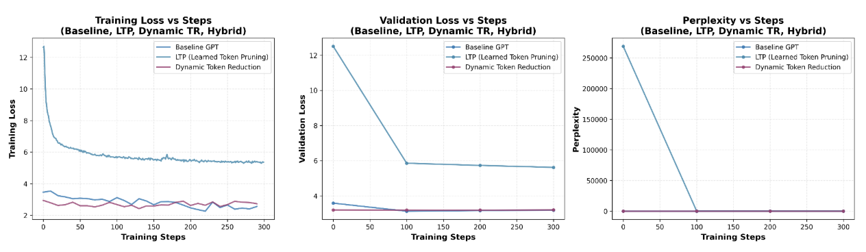
Figure 1 shows the training progression for all 300 training steps plotted against training loss, validation loss, and perplexity. The baseline exhibits stable training starting off with around a 3.6 training and validation loss and decreases smoothly to 3.3 with a corresponding perplexity of 22.
Dynamic TR also has relatively stable training behavior due to freezing the GPT-2 backbone during policy training. The training and validation loss hovers around 3 and ends off at 3.4. Since the perplexity graph through training remains relatively low and flat, stabilizing around 30, this means DTR's policy networks learn to make policy decisions without degrading model performance.
In contrast, LTP has significantly more unstable training. Training and validation loss starts off around 13 and eases down to right below 6, at around 5.8 validation loss after 300 training steps. The perplexity plot reveals that LTP's perplexity starts off high around 270,000, mirroring the high loss values before plateauing to 330. This suggests that jointly training the LTP with the backbone causes the model to enter into a less stable loss landscape.
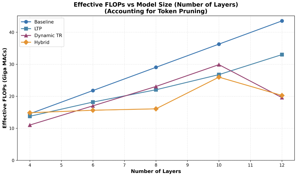
Computational efficiency vs. model depth
Figure 2 shows how the compute cost scales with changes in model size. We can see that the baseline increases linearly with model size, which is expected. We also see that our pruning strategies are all below the baseline, meaning we save compute for all. We notice that the DTR and Hybrid models prune more aggressively with the more layers we add. This means that adding more than 12 layers has diminishing returns on compute cost.
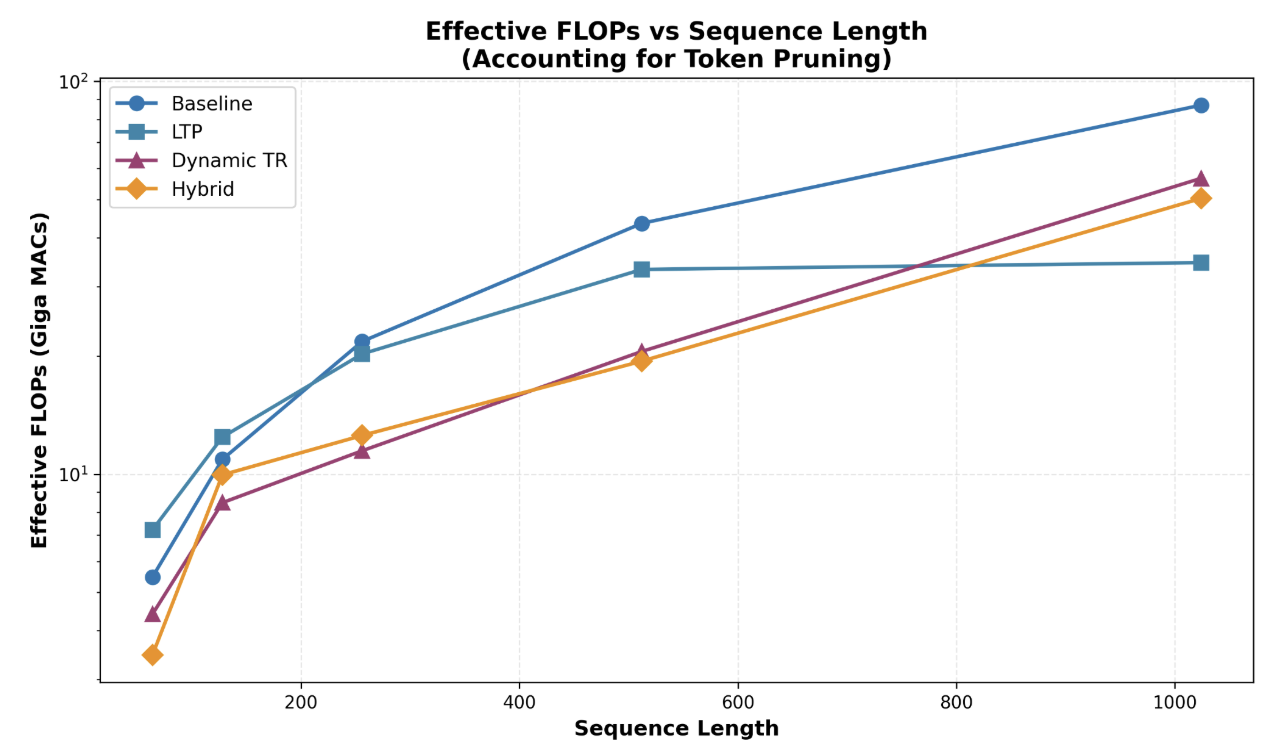
Computational Efficiency vs. Sequence Length
Figure 3 shows how each method handles quadratic attention as the sequence length grows. All models share a common trend that as sequence length increases, so do the effective FLOPs. The hybrid model has the lowest effective FLOPs among all models until sequence length 1024, which has LTP as the lowest amount of effective FLOPs. LTP's curve flattens significantly after sequence length 512 because longer sequence lengths contain more redundant tokens that receive low attention scores. The computational benefits of pruning seem to be more prominent under long sequence lengths.
Perplexity vs. Sequence Length
In Figure 4, we expose the weakness of combining different pruning methods into a hybrid model. The baseline and Dynamic TR model achieves consistent perplexity and decreases with sequence length. However, LTP and hybrid approaches are much more unstable with perplexity increasing with increasing sequence length. At sequence length 64, LTP perplexity starts off around 50 but as the length increases to 256, it explodes to nearly 300 before recovering to 250 at length 512. This means that freezing the backbone weights causes the model to place more emphasis on the pruning objective at the expense of language modeling. The hybrid model has the highest perplexity among all models and sequence lengths, starting off at around 50 and increasing to over 4,000. The hybrid architecture seems to compound errors from early pruning by DTR, which removes tokens later that LTP in later layers would have needed.
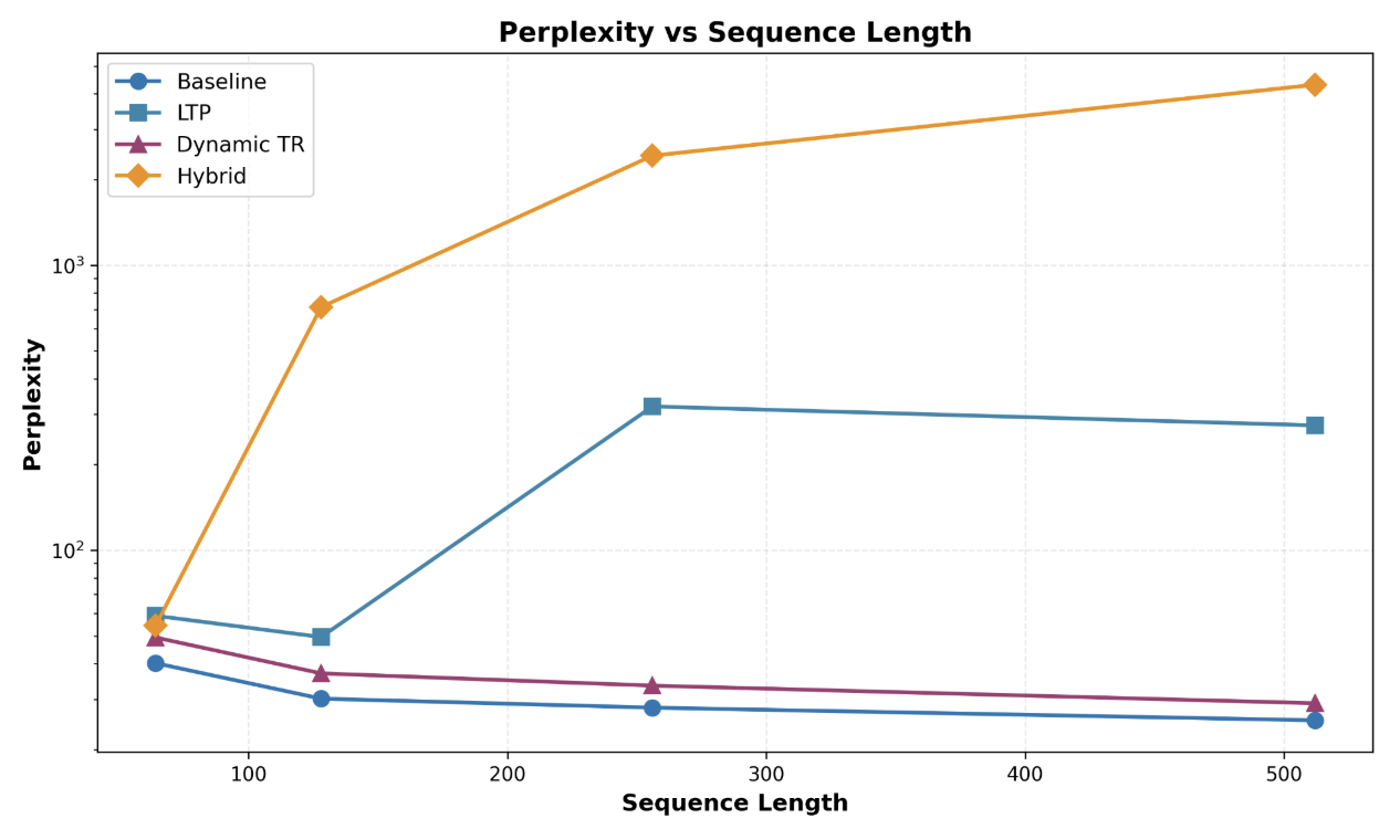
The results reveal the tension of integrating pruning methods fit for encoder only models into autoregressive decoder models. Dynamic TR achieves the best trade off, providing computational savings with FLOPs while maintaining performance with minimal perplexity degradation. Encoder models like BERT have context of all words in a sequence, meaning previous and future tokens can attend to the current token. In contrast, autoregressive models use a causal mask that prevents future tokens from attending to the current token, which is likely to explain LTP and hybrid approaches' poor performance, suggesting that attention-based importance scoring on causal masks are poorly suited for pruning.
Conclusion
In this project we have shown that effective pruning strategies can be applied successfully to autoregressive models. We also provided insight on how two different learning methods, reinforcement and supervised, can be combined to create effective pruning to save computation cost. Although our pruning methods did not perform how we wanted, we still believe that token pruning is an effective method for improving efficiency.
Limitations
Our study had several limitations that contextualize our findings. A limitation for this project was our access to hardware. We only had access to one GPU, so we had to choose a small fine-tuning dataset, which may have contributed to overfitting on GPT-2. Larger datasets provide stronger training signals and help with the model learning process to learn more meaningful thresholds and policies.
Another limitation was hyperparameter sensitivity. We believe given more time we would have been able to figure out how to improve efficiency while preserving performance through better selection of hyperparameters.
Future Works
For our future works we want to experiment more with how different hyperparameters affect performance during fine-tuning. If we had more hardware for computation, we would want to use a larger model for these experiments. We would also want to increase the size of our dataset, which might reduce overfitting early on in fine-tuning. One more experiment we would like to implement is changing our importance score calculation for LTP to account for causal masking.
References
- Ashish Vaswani, Noam Shazeer, Niki Parmar, Jakob Uszkoreit, Llion Jones, Aidan N. Gomez, Łukasz Kaiser, and Illia Polosukhin. 2017. Attention is all you need. In Advances in Neural Information Processing Systems 30 (NeurIPS 2017), I. Guyon, U. V. Luxburg, S. Bengio, H. Wallach, R. Fergus, S. Vishwanathan, and R. Garnett (Eds.). Curran Associates, Inc., 5998–6008. https://arxiv.org/abs/1706.03762
- Paul Michel, Omer Levy, and Graham Neubig. 2019. Are sixteen heads really better than one? In Advances in Neural Information Processing Systems 32 (NeurIPS 2019), H. Wallach, H. Larochelle, A. Beygelzimer, F. d'Alché-Buc, E. Fox, and R. Garnett (Eds.). Curran Associates, Inc., 14014–14024. https://arxiv.org/abs/1905.10650
- Yichong Leng, Chen Zhang, Junru Chen, Xiaohui Wang, Shiyu Chang, Yifan Gong, Rong Jin, and Linquan Zhang. 2024. Vocabulary pruning for efficient fine-tuning of large language models. arXiv preprint arXiv:2410.18952 (2024). https://arxiv.org/abs/2410.18952
- Zhuohan Li, Eric Wallace, Sheng Shen, Kevin Lin, Roberto Calandra, Kurt Keutzer, and Joseph E. Gonzalez. 2021. Learned Token Pruning for Transformers. arXiv preprint arXiv:2107.00910 (2021). https://arxiv.org/abs/2107.00910
- Ji Xin, Raphael Tang, Yaoliang Yu, and Jimmy Lin. 2021. TR-BERT: Dynamic token reduction for accelerating BERT inference. In Proceedings of the 2021 Conference of the North American Chapter of the Association for Computational Linguistics: Human Language Technologies (NAACL-HLT 2021). Association for Computational Linguistics, 5798–5809. https://arxiv.org/abs/2105.11618